15. Generic Transformations

The previous chapters describe how one may do various unary or binary operations over your data, apply symmetry operations or build analytical model and simulate it over whole sqw file. As whole sqw file can not be generally placed in memory, all these operations are based on special PageOp family of algorithms, which operate loading a page of data in memory and applying various operations to these data. For unary, binary and symmetry operations we wrote these transformations for users and the sqw_eval algorithm from Simulation section gives user a set of rules to write his own model in hklE coordinate system and apply it to whole sqw object.

15.1. Introduction

Generic transformations are the set of algorithms, which give user access to the body of PageOp algorithm to do whatever he needs with his sqw data. As this gives user the most flexible access to modifying sqw data, it requests from user most knowledge of sqw object design to do useful things with these data.

In particular, user have to know, that Horace stores its pixel data in Crystal Cartesian coordinate system, which is orthogonal coordinate system attached to crystal lattice with x-axis parallel to a* inverse lattice vector and two other axis being orthogonal to it. He needs to write transformations over page of data presented in the form of [9 x npix] matrix, where npix is the page size (defined by hor_config.mem_chunk_size value), each column corresponds to a pixel and the pixel contain the following values:

row 1: u1                 % first momentum transfer (Q_x) coordinate in A^-1
row 2: u2                 % second momentum transfer (Q_y) coordinate in A^-1
row 3: u3                 % third momentum transfer (Q_z) coordinate in A^-1
row 4: dE                 % energy transfer values  (meV)
row 5: run_idx            % identifier of the run, contributed into this pixel
row 6: detector_idx       % indices of the detectors, contributing into the image
row 7: energy_idx         % indices of energy transfer values registered in experiment
row 8: signal             % signal (normalized number of neutron events) registered for this pixel
row 9: variance           % variance of the signal above.

In addition to that user should be familiar with the definition of projection, which establishes relationship between pixel coordinate system and the image coordinate system. A projection has number of methods from which two the most useful for transformations are:

% Transform pixels expressed in crystal Cartesian or any source
% coordinate systems defined by projection into image coordinate system
[pix_transformed] = proj.transform_pix_to_img(pix_cc);
% Transform pixels expressed in image coordinate coordinate systems
% into crystal Cartesian system or other source coordinate system,
% defined by projection
[pix_cc] = proj.transform_img_to_pix(pix_transformed);

Where proj is usually projection used by sqw object of interests, pix_cc is [4 x npix] matrix of pixel coordinates expressed in Crystal Cartesian coordinate system (see four first rows of pixels data above) and pix_transformed is [4 x npix] array of pixels coordinates expressed in image coordinate system.

Finally user should be familiar with concept of object oriented programming as to write custom transformation one needs to use properties of the core transformation classes PageOp_sqw_op or PageOp_sqw_op_bin_pixels described below alongside with the description of the appropriate algorithm.

15.2. sqw_op algorithm

sqw_op is the algorithm, which provides user with opportunity to modify signal and error values and perform multiple unary or binary operations simultaneously while transforming large sqw object. Its signature looks as follows:

wout = sqw_op(win, @sqw_op_func, pars)
wout = sqw_op(win, @sqw_op_func, pars,'outfile',target_file_name)

where:

• win – sqw file, cell array array of sqw objects or strings that provides filenames of sqw objects on disk serving as the source of sqw data to process using sqw_op_func

• @sqw_op_func – handle to a function which performs desired operation over sqw data.

• pars – cellarray of parameters used by sqw_op_func. If sqw_op_func have no parameters, empty parentheses {} should be provided.

Optional:

• "outfile" – key followed by the string, which defines the name or name with full path to the file to store resulting filebacked sqw object. If one does not specify this, the resulting filebacked object will be temporary, i.e. will be deleted after variable wout will go out of scope.

The output is:

• wout: an sqw object built from win by applying sqw_op_func over all pixels of win objects and calculating appropriate image averages.

@sqw_op_func should have the form:

function output_sig_err = sqw_op_func(in_page_op,parameters)

   data = in_page_op.data; % get page of pixel data expressed in Crystal Cartesian coordinate system
   % Operations over signal and error as function of in_page_op, data and other parameters
   ...
   % return results of operation as [2 x npix ] array of modified signal and variance data
   output_sig_err = [signal_calc(:)';error_calc(:)'];
end

where in_page_op is the instance of PageOp_sqw_op class which is the core of sqw_op algorithm and will provides user with access to page of pixels data and other properties, necessary to define proper transformation.

Now let’s assume that you want to multiply an sqw object by 2 and extract a constant from the obtained value. You can do that using unary and binary operations, described in the chapter above:

>>wout = 2*w_in - 1;

This is simple code, but if your objects are filebased, this will requests two scans over large sqw object. If you write sqw_op_func function:

function output_sig_err = sqw_op_unary(in_page_op,varargin)
   % Apply two simple transformations of signal of an sqw object in one go.

   data = in_page_op.data;       % get access to page of pixel data
   data(8,:) = 2*data(8,:)-1;    % change pixel data signal by multiplying it by 2 and extracting 1
   output_sig_err = data(8:9,:); % extract signal and unchanged error into form, requested by algorithm
end

and apply sqw_op algorithm:

wout = sqw_op(win, @sqw_op_unary, 'outfile','operations_result.sqw')

You can do the same operation over large filebacked sqw object in one scan over whole sqw file, which in this simple case will be two times faster then applying these operations one after another.

If your theoretical model is built in Crystal Cartesian coordinate system rather than in hkldE coordinates you may write and apply it to pixel coordinates exactly like hkldE model for sqw_eval algorithm. Here, as the example of using sqw_op we try to remove cylindrical background obtained in the diagnostics chapter of this manual. It may be not the best way of removing whole background but a good example of using special projection to transform data expressed in Crystal Cartesian coordinate system to image coordinate system.

The sample background present in this case may be estimated by running Mantid reduction script and adding all reduced runs together:

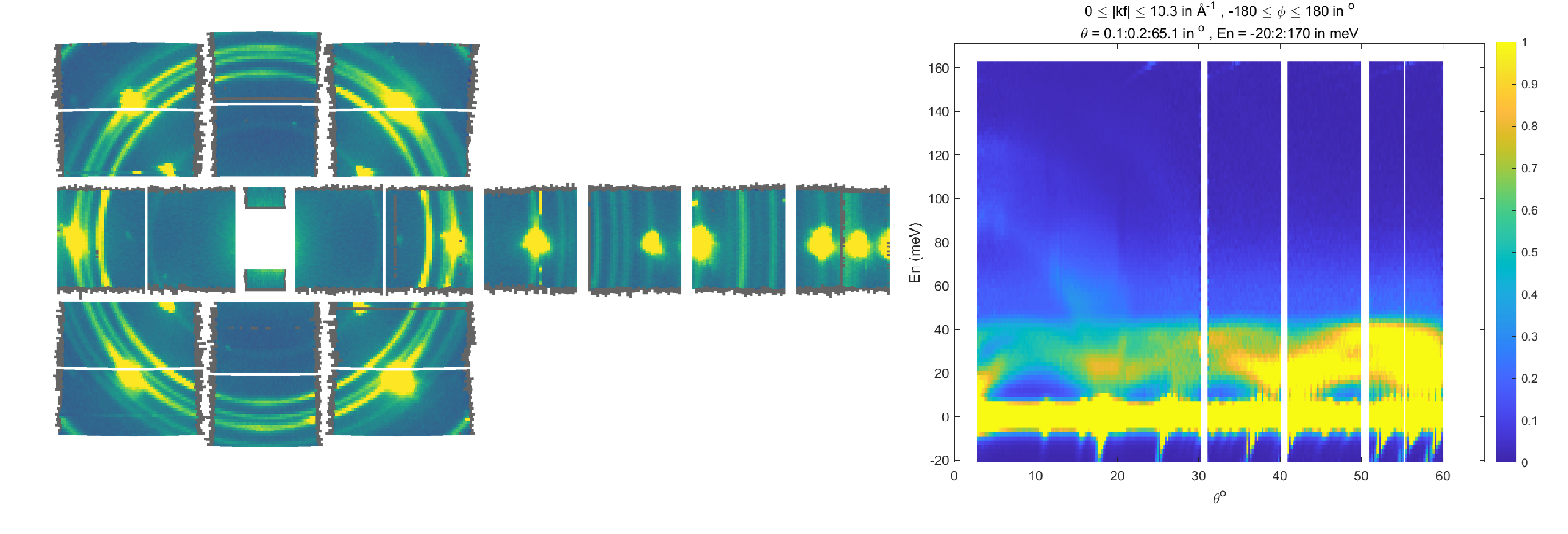
Left part of the image represents Mantid instrument view image. It is obvious that there is small beam leakage around beam stop window and strong powder lines around Bragg peaks. This is the background which one wants to remove. Right part of this image represents 2-dimensional image obtained from instrument_view_cut and we want to extract this image from whole sqw file containing magnetic signals.

Slim-lined script which would produce such background removal is provided below:

%%=============================================================================
%       Calculate and remove background for Ei=200 meV sample dataset
% =============================================================================
% Get access to sqw file for the Ei=200meV containing Horace angular scan
% which is located in "sqw/sqw2024" folder, in the position relative to the
% location of the script.
root_dir = fileparts(fileparts(fileparts(mfilename("fullpath"))));
sqw_dir=fullfile(root_dir,'sqw','sqw2024');

% define the name of the source file and the name of the resulting data file.
data_src200 =fullfile(sqw_dir,'Fe_ei200_align.sqw');
target = fullfile(sqw_dir,'Fe_ei200_no_bg2D.sqw');
src200 = sqw(data_src200); % create filebacked source sqw object

% calculate 2-dimensional cylindrical background in Instrument coordinate system.
w2_200meV  = instrument_view_cut(src200,[0,0.2,65],[-20,2,170]);

% build background model for interpolation expressed in
% instrument view coordinate system.
x1 = w2_200meV.p{1};
x2 = w2_200meV.p{2};
x1 = 0.5*(x1(1:end-1)+x1(2:end));
x2 = 0.5*(x2(1:end-1)+x2(2:end));
F = griddedInterpolant({x1,x2},w2_200meV.s); % define background model using linear
% interpolation of signal

% call sqw_op with function to remove background
src200_noBb = sqw_op(src200,@remove_background,{w2_200meV,F},'outfile',target);

The page-function with actually used to remove background in the code above is:

function sig_var = remove_background(pageop_obj,bg_data,bg_model,varargin)
    % function to remove background from page of data.
    % Inputs:
    % pageop_obj -- instance of PageOp_sqw_op class providing necessary page of pixels data
    % bg_data    -- two dimensional background dataset to remove
    % bg_model   -- gridded interpolant to calculate background signal on 2-Dimensional
    %               image.
    % Returns:
    % sig_var     -- 2xnpix array of modified pixel's signal and variance.

    data  = pageop_obj.page_data; % get access to page of pixel data

    % 2D background. get access to kf_sphere_proj to transform pixel data
    % into instrument coordinate system where background is
    % defined using instrument view projection
    % As this is special projection, it needs 5 rows of pixel data (needs run_id)
    % rather then the standard projection, which takes 4 rows.
    pix   = bg_data.proj.transform_pix_to_img(data(1:5,:)); % you may define your own
    % complex transformation to convert pixels from Crystal Cartesian coordinates to
    % image coordinates, but here you have your projection already defined to do that.

    % interpolate background signal on the pixels coordinates expressed
    % in instrument coordinate system.
    bg_signal = bg_model(pix(2,:),pix(4,:));

    % retrieve existing signal and variance values
    sig_var = data([8,9],:);
    % remove interpolated  background signal from total signal
    sig_var(1,:) = data(8,:)-bg_signal;
    % exclude negative results from possible future fitting routine
    over_compensated = sig_var(1,:)<0;
    %sig_var(1,over_compensated) = 0;
    sig_var(2,over_compensated) = 0;

end

Modified image clearly shows substantial decrease in parasitic signal around elastic line:

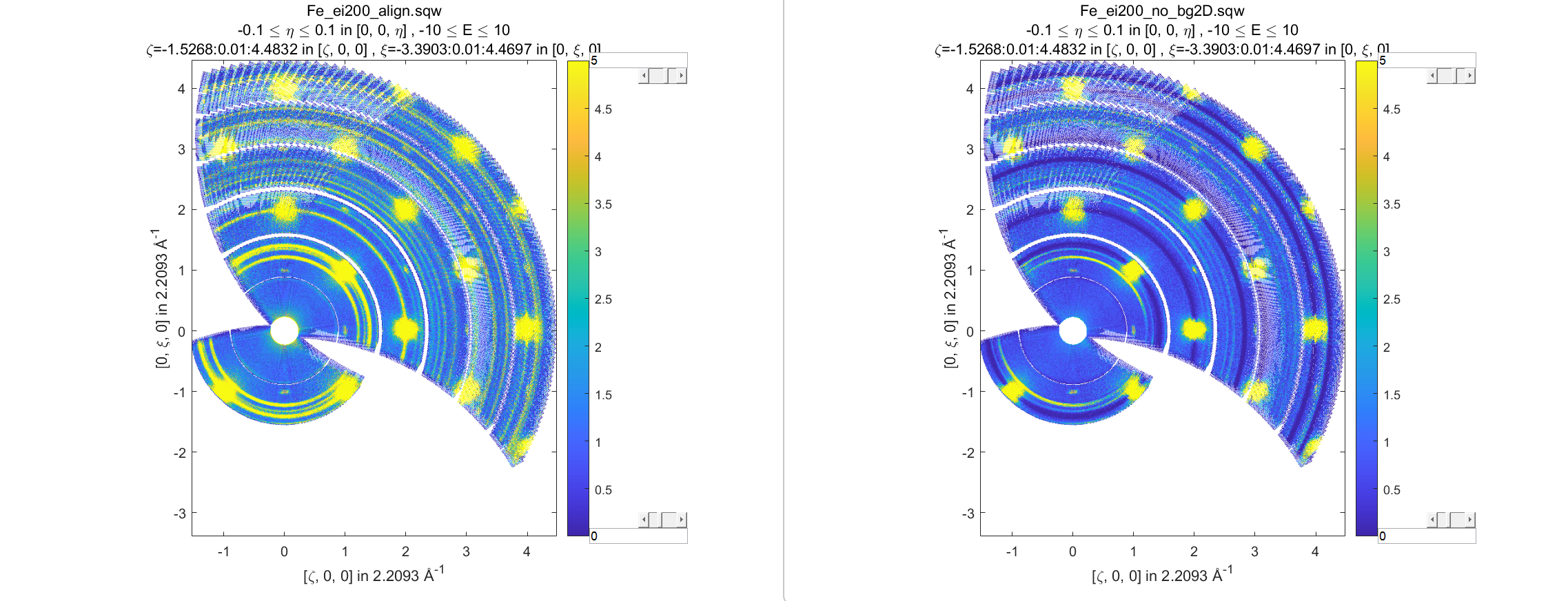
Better background model is possible to remove more parasitic signal, though this task is fully in the hands of user.

15.3. sqw_op_bin_pixels algorithm

Let’s assume you are interested in magnetic signal which is present at relatively low \(\|Q\|\) due to magnetic form factor and signal covers multiple Brillouin zones at low \(\|Q\|\). You want to accumulate magnetic signal in first Brillouin zone to increase statistics and consider everything which is beyond some specific \(\|Q\|\) - value to be background to remove as signal there is negligibly small due to magnetic form factor, so you also want to move this signal to first Brillouin zone and extract background from the magnetic signal. Figure below give example of such situation:

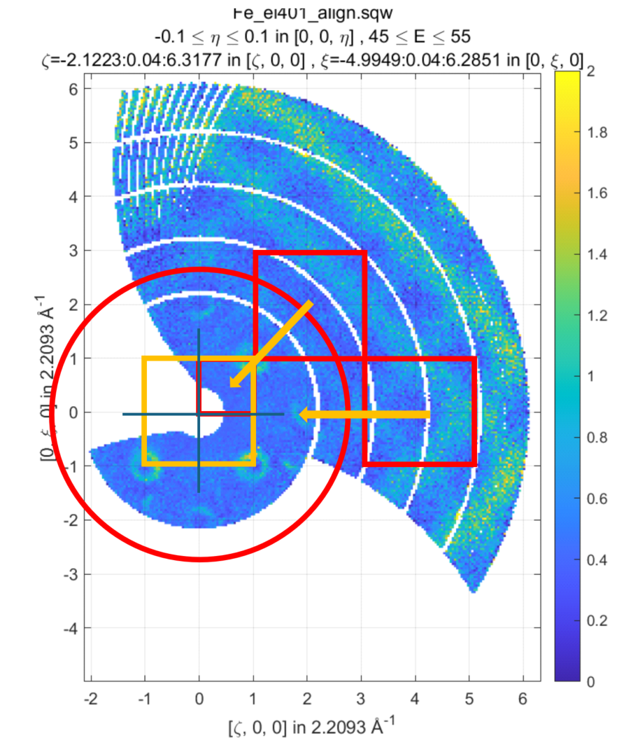
Sample differential cross-section measured on MAPS and showing magnetic signal within read-cycle surrounded area and background signal (phonons) inside and outside of this area. Yellow box represents double-size Brillouin zone where data moved using shift operation and its top right quadrant – the area where data should be finally moved using folding and reflection.

sqw_op algorithms would not allow you to do this, as you can not change pixels coordinates alongside with everything else. sqw_op_bin_pixels algorithm is written to allow user changing pixels coordinates. Its interface is the mixture of sqw_op interface and cut interface, which defines construction of new image of interest from provided pixel and image data:

wout = sqw_op_bin_pixels(win, @sqw_op_func, pars,cut_pars{:})
wout = sqw_op_bin_pixels(win, @sqw_op_func, pars,cut_pars{:},'outfile',target_file_name);

where:

• win – sqw file, cell array array of sqw objects or strings that provides filenames of sqw objects on disk serving as the source of sqw data to process using sqwop_func

• @sqw_op_func – handle to a function which performs desired operation over sqw data.

• pars – cellarray of parameters used by sqw_op_func. If sqw_op_func have no parameters, empty parentheses {} should be provided.

• cut_pars – cellarray of cut parameters as described in cut except symmetry operations which are not supported by this algorithm as cut parameters but may be customized and provided as the parameters of sqw_op_func.

Namely, cut_pars have the form:

cut_pars ={[ proj], p1_bin, p2_bin, p3_bin, p4_bin[, '-nopix']};

where:

• proj defines the axes and origin of the cut including the shape of the region to extract and the representation in the resulting histogram. If not provided, the projection is taken from the input win object.

• pN_bin describe the histogram bins to capture the data. In details they described in the chapter about binning arguments

• optional '-nopix' argument means that resulting object would be dnd object, i.e. object which does not contain pixels.

@sqw_op_func for sqw_op_bin_pixels algorithm have form similar to the one used by sqw_op algorithm, except it should return full page of modified pixels data:

function output_data = sqw_op_func(in_page_op,parameters)

   data = in_page_op.data; % get page of pixel data expressed in Crystal Cartesian coordinate system
   % Operations over signal and error as function of in_page_op, data and other parameters
   ...

   % return results of operation as [9 x npix ] array of modified pixels data, where all
   % values of the array may change.
   output_data = modify_data(data,parameters{:});

end

Slim-lined script to calculate background in the situation, described on the figure above looks like that:

%%=============================================================================
%       Calculate background for Ei=400 meV
% =============================================================================
% Get access to sqw file for the Ei=400meV Horace angular scan
root_dir = fileparts(fileparts(fileparts(mfilename("fullpath"))));
sqw_dir=fullfile(root_dir,'sqw','sqw2024');

data_src400 =fullfile(sqw_dir,'Fe_ei401_align.sqw');
target = fullfile(sqw_dir,'Fe_ei401_noBg_4D_reducedBZ_FF_ignored.sqw');

% initialize source filebacked object to operate over
src400 = sqw(data_src400);

alatt = src400.data.alatt;  % get access to lattice parameters
angdeg= src400.data.angdeg; % and lattice angles
rlu = 2*pi./alatt;          % calculate reciprocal lattice (case of cubic lattice)
r_cut2 = (3.5*rlu(1))^2;    % define cut-off radius for background
old_range = src400.data.axes.get_cut_range(); % obtain binning for existing object
del = 0.05;                 % define new binning for q-coordinates
zoneBins = [-del,0.05,1+del];
e_bins = old_range{4};      % retain existing binning for energy coordinates

% define cut ranges
cut_range = {zoneBins *rlu(1),zoneBins*rlu(2),zoneBins*rlu(3),[-15,2,340]};

bg_file = 'w4Bz_400meV_bg.mat'; % where we want to save our background

% run sqw_op_bin_pixels to calculate background in the first Brillouin zone.
sqw400meV_Bz_bg = sqw_op_bin_pixels(src400, @build_bz_background, {r_cut2,rlu},cut_range{:},'-nopix');  %
sqw400meV_Bz_bg.filename = 'sqw400meV_Bz_bg'; % redefine name of the resulting dnd object
save(bg_file,'sqw400meV_Bz_bg');   % save result for further usage.

Where the function to calculate background is:

function data = sqw_op_build_bz_bckgrnd(pageop_obj,r2_ignore,rlu)
%sqw_op_build_bz_bckgrnd calculates background signal from scattering function
% taken at of q-values beyond of the specified cut-off radius
% and moves background signal into first Brilluoin zone.
%
% Inputs:
% pageop_obj -- Initialized instance of PageOp_sqw_op_bin_pixels object providing all necessary data
% r2_ignore  -- square of cut-off radius to select background (A^-2)
% rlu        -- reciprocal lattice vectors for the used lattice

% Get access to [9 x Npix] page of pixels data
data = pageop_obj.page_data;
% calculate pixels distances from centre of Crystal Cartesian coordinate system
Q2 = data(1,:).*data(1,:)+data(2,:).*data(2,:)+data(3,:).*data(3,:);
keep = Q2>=r2_ignore; % background % identify pixels outside of cut-off radius
%keep = Q2<r2_ignore;   % foreground
data = data(:,keep);  % select pixels outside of cut-off radius
if isempty(data)
    return;    % leave if this page does not contain background data
end
% Cubic lattice scale in BCC lattice
scale = 2*rlu;
q_coord = data(1:3,:);
img_shift   = round(q_coord./scale(:)).*scale(:); % BRAGG positions
% in the new lattice are located at the even rlu values
% move all q-coordinates into expanded Brillouin zone +-1*rlu size
q_coord  = q_coord - img_shift;

% move 7 cubes with negative coordinates of expanded Brillouin zone into the first cube.
invert = q_coord<0;
q_coord(invert) = -q_coord(invert);

% construct result containing modified coordinates
data(1:3,:) = q_coord;

end

Note that the function returns full [9x N] page of pixel data, where N is smaller then input number of pixels. Rows 12-13 of the function above distinguish between background and foreground. As one can see, difference is just in taking signal for background outside of the cut-off radius and foreground – inside of cut-off radius. This causes visible magnetic foreground signal contributing into background, but as this signal is smaller then 10% of foreground signal, here we ignore it, bearing in mind that this correction may be calculated more accurately and applied to final results.

All these considerations and their significance or non-significance are case-specific user have full control and responsibility for writing his own background/foreground function and interpreting results, obtained using this function.

Figure below shows sample background calculated using sqw_op_bin_pixels algorithm and background-calculating function sqw_op_build_bz_bckgrnd.mat provided above. The background extraction is also performed using sqw_op_bin_pixels algorithm as it combines moving foreground signal into first Brillouin zone, background extraction, Magnetic form-factor corrections and parasitic signal removal. As this is relatively complex user function based on elements, provided above, we do not provide script to obtain this result in the document but placed the script which does these operations (sqw_op_move_to_bz0_and_remove_bckgrnd.mat) into Horace/example/ folder.

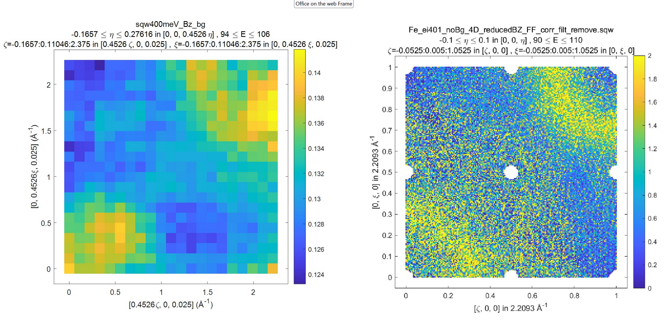
Background and Foreground signals for data demonstrated at the beginning of this chapter. Note the difference in intensity scale between background and foreground signals.

Round holes in the corners, centre and middle-edges of the foreground scattering function are related to the procedure of suppression of the parasitic reflections in [0,0,1] direction from cubic sub-lattice of the sample. The piece of code responsible for this suppression and the holes is marked and highlighted within the sample code.

Note

sqw_ob_bin_pixels is the algorithm acting on full sqw object. As such, it is not particularly fast until it parallel implementation is available. The examples, provided here are done for whole sqw object, located on file, so the pictures show 2-dimensional cuts of full 4-dimensional filebacked object. It is recommended to debug user functions on 2-dimensional cuts/objects located in memory before running long calculations on full 4-dimensional object.

15.4. sqw_op_bin_pixels algorithm with "-combine" option

Normally sqw_op_bin_pixels algorithm applied to cellarray of sqw objects or sqw files will apply specified sqw_op_function to each input sqw object. If you invoke this algorithm with "-combine" option, it will combine all input objects into single object with coordinate system defined by the first input object.

We extracted description of "-combine" option into separate chapter due to close connection between the sqw_op_bin_pixels with the sample function described below within cut in Cut with symmetry operations, described in chapter Symmetry Operations. The code of the sample function below substantially overlaps with the code used in the core cut with SymOp symmetrisation algorithm.

The similarities and differences between these two algorithms are summarized in the table:

Number	Action	cut with SymOp	sqw_op_bin_pixels with "-combine"
1	Cuts source:	single sqw obj with cuts generated by symmetry operations	random selections of sqw cuts, may be from different sqw objects
2	Multiple transformations applied to single data	Not allowed	simple modifications to standard script
3	Include same pixels from multiple symmetry op.	No. Efficient exclusion algorithm	request complex coding. Probably not very efficient but possible.
4	Possibility to perform other operations alongside with symmetry.	No	Possible
5	User efforts	Average	High

In more details the table above can be expanded as follows:

1. cut with SymOp generates number of cuts related by symmetry operation and combine data from these cuts together. You have to provide sqw_op_bin_pixels with set of cuts (related by symmetry operations or not related – its your choice) and then these cuts are combined together exactly in the same way as in cut with SymOp. As the consequence, cut with SymOp will work with single sqw file, and cuts provided to sqw_ob_bin_pixels can be taken from multiple sqw files.

2. Let’s assume you transform data defined in range [-1:-3] into range [0:1] using folding operations around axes passing through points 0 and 1. If you use cut with SymOp, the data reflected from range [1:3] will be reflected into range [-2:1] and the data block [-2:0] will be dropped by cut ranges. reflected. This is the consequence of using the current implementation of the algorithm, which eliminates double counting of the same data transformed multiple times using multiple symmetry operations. If you need to keep these data, you need to use sqw_op_bin_pixels with properly modified custom sqw_op_function.

3. cut with SymOp carefully cares about error counting not to double-count the same pixels, transformed multiple times by different symmetry operations. As data in SymOp may come from multiple sources, its very difficult to implement such algorithm for sqw_op_bin_pixels. This may be done with some efforts from user (e.g. by calculating unique pixel id and comparing pixels usage) but this algorithm does not look very efficient.

4. As user expects to write his own sqw_op_function he may use multiple transformations of his choice to modify combined data. cut with SymOp intended for performing operations performed by well defined SymOp classes.

5. Summarizing all above, one can say that cut with SymOp is intended for simple combining of symmetry-related cuts, while sqw_op_bin_pixels gives user wider opportunities, allows combining much wider range of data but requests from user more experience with MATLAB programming and better knowledge of Horace internal structure.

Simplest form of the function, which allows combining multiple cuts into single cut is:

function result = move_all_to_proj(pageop_obj,proj_array,varargin)
% Convert all equivalent directions found in the cellarray of input datasets into
% the coordinate system specified by pageop_obj.
%
% Inputs:
% pageop_obj  -- instance of PageOp_sqw_binning object containing
%                information about source sqw object(s), including page of
%                pixel data currently loaded in memory, projection, which
%                defines target coordinate system and the target image
%                to convert all input data in.
% proj_array  -- array of projections which describe directions of cuts
%                to combine.
%
% Returns
% result      -- page of modified pixels data to bin using
%                PageOp_sqw_binning algorithm transformed into coordinate
%                system related with first projection
%
%

% Get access to [9 x Npix] page of pixels data
data = pageop_obj.page_data;
% get access to the projection, which describes target image
targ_proj = pageop_obj.proj;
%
% done explicitly for 2-D cuts for performance to avoid internal loop over pixels ranges
%---------------------------------------------------------------------------------------
% Get access to the target image and obtain indices of the integration axis
iax  = pageop_obj.img.iax;  % expect two integration axis here
% get cut ranges of the image to combine everything into these ranges
cut_range = pageop_obj.img.img_range(:,iax  );
%
q_coord = data(1:3,:);
result = cell(1,numel(proj_array));
% go through all combining images coordinates system, converting appropriate pixels
% into coordinate system, related to target projection
for i=1:numel(proj_array)
    % input projections used for cut do not have lattice set up for them.
    % They need lattice to be fully defined and use projection methods so let's set it up here.
    % may be taken out of loop for performance though it is fast anyway.
    proj_array(i).alatt = targ_proj.alatt;
    proj_array(i).angdeg = targ_proj.angdeg;
    % transform momentum transfer values from current page of data into
    % image associated with proj_array(i) projection
    coord_tr = proj_array(i).transform_pix_to_img(q_coord);
    % find the data falling outside of the target image range
    % forcing target image and the image produced by current projection to
    % coincide.
    include = coord_tr(iax(1),:)>=cut_range(1,1)&coord_tr(iax(1),:)<=cut_range(2,1)&...
        coord_tr(iax(2),:)>=cut_range(1,2)&coord_tr(iax(2),:)<=cut_range(2,2);
    % extract coordinates which lie within current cut ranges.
    coord_tr  = coord_tr(:,include);
    res_l = data(:,include);
    % transform pixels coordinates from image defined by proj_array(i) cut
    % projection into the Crystal Cartesian coordinates system related with
    % target projection.
    res_l(1:3,:) = targ_proj.transform_img_to_pix(coord_tr);
    % collect transformed pixels as partial result
    result{i} = res_l;

    data = data(:,~include); % extract remaining data for processing using
    % other projections.
    if isempty(data) % leave if all data was processed and transformed
        break
    end
    q_coord = data(1:3,:);
end
% combine all partial cut results
result = cat(2,result{:});
end

The original of this function is located in Horace/example/ folder. The details of the implementation are provided in the comments to the function. The main idea of the operation is that you select one main cut and combine all additional images forcefully “overlapping” images one over another transforming pixels coordinates accordingly.

Image below shows the way to overlapping two cuts together and the result of such overlapping.

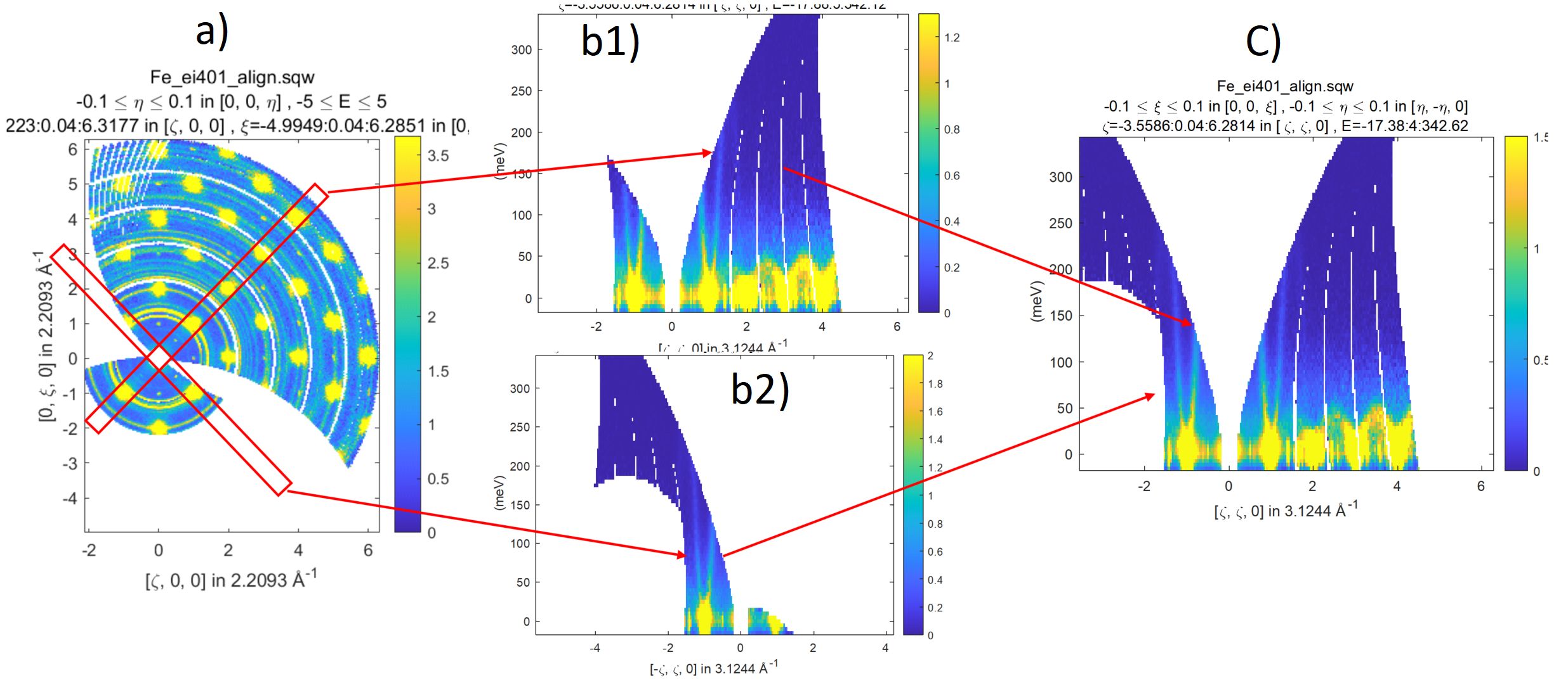
Overlap two cuts demonstrated on the left image, display them (central image) and combine together using sqw_op_bin_pixels algorithm with combine function above.

Simple script which allows to produce result presented on the right side of picture above (image (c) ) from the data on the left side of the image above using sqw_op_bin_pixels and combine function above looks as follows:

source = sqw('source_file_name');  % define filebacked source sqw object
w2 = cut(line_proj,[],[],[-0.1,0.1],[-5,5],'-nopix');
plot(w2)    % plot image (a)
proj1 = line_proj([1,1,0],[-1,1,0]);
proj2 = line_proj([-1,1,0],[1,1,0]);
cut_ranges = {[],[-0.1,0.1],[-0.1,0.1],[-10,5,360]};
cut1  = cut(source,proj1,cut_ranges{:});  % cut sqw object presented on image b1)
cut2  = cut(source,proj2,cut_ranges{:});  % cut sqw object presented on image b2)
% combine cut1 and cut2 together producing final result.
wout  = sqw_op_bin_pixels({cut1,cut2},{[proj1,proj2]},proj1,cut_ranges{:},'-combine');
plot(wout); % plot image c)